How Weather Shapes Air Pollution in the United States

Air quality is measured in terms of Air Quality Index (AQI), which are different values that determine quality of the air. Air pollution is the contamination of the air compared to its normal state with air pollutants such as PM2.5 (Particulate Matter 2.5, with 2.5 micrometers being the particle size of the air pollutant). AQI values ranging from 0-50 (PM 2.5 concentration being micrograms per cubic meter (μg/m3)) are satisfactory with almost no risk of 24- hour exposure to PM2.5 (PurpleAir, Inc. Real-time air quality monitoring by PurpleAir). Air quality is acceptable in levels of 51-100 μg/m3, but as AQI ranges rise, health risks increasingly worsen and affect sensitive individuals. Levels of air quality ranging from 100-150 μg/m3 affect members of sensitive groups by potentially damaging their health within 24 hours of exposure, although the general public remains mainly unaffected. Sensitive groups include individuals with present or past asthma, respiratory infections, and more (Spickett, 2024). AQI levels ranging from 151-200 μg/m3 are unhealthy, and from 201-300 μg/m3 are very unhealthy. However, any exposure greater than 300 μg/m3 can negatively affect the entire population if they are exposed for a cumulative of 24 hours or more. Even though the general population is not often exposed to levels like these, groups that have a higher sensitivity to pollutants in the air are nonetheless affected.

The burden and severity of exposure to PM2.5 are based on the duration and concentration of the exposure (Daouda et al., 2022). Racial/ethnic disparities in nationwide PM2.5 concentrations: Perils of assuming a linear relationship. Environmental Health Perspectives, 130(7). An increase in exposure can lead to an increase in symptom severity and multiple negative health effects, having an immense impact on the lives of civilians (Larr et al., 2016). For instance, damage to the respiratory and cardiovascular systems, impairments to memory functions, and increased risk of cancer in the body are all within the scope of PM2.5-caused illnesses (Liu, J., et al., 2021). Disparities in air pollution exposure in the United States by race-ethnicity and income, 1990–2010. People of all ages can be affected by particulate matter, with particularly severe effects on the elderly, children, and pregnant women. When exposed to enough air pollution at a young age, severe respiratory illnesses can develop, worsen, or even kill the child as they grow (Manisalidis et al.). In fact, the World Health Organization estimated that 4.2 million premature deaths occur per year because of exposure to ambient, outdoor air pollution (Spickett, 2024). This illustrates the urgent need for air quality management.

Even with low levels of AQI, unhealthy exposures to particulate matter significantly affect human health, which is why it is so important to understand what correlates with particulate matter. While previous studies have examined the general health effects of PM2.5, it is important to understand what impacts AQI by analyzing the correlation between air quality levels and meteorological factors such as temperature, air pressure, and humidity. If air pollution and the most exposed groups are understood on a deeper level, New York City – a place particularly impacted by particulate matter pollution while also having diverse climatic factors ((New York State Department of Environmental Conservation. (n.d.). Home.)) – and the United States nationally can make greater strides towards more viable reforms to improve air quality ((Education, UCAR Center for Science. (2024b). Extreme events and human health. Center for Science Education.)). Across five continents, rising respiratory diseases have been found in cities with increased pollution (Education, UCAR Center for Science. (2024). How weather affects air quality. Center for Science Education.). In attempts to counter the negative effects of air quality, the Environmental Protection Agency (EPA) passed the Clean Air Act of 1970 (CAA) to limit the amount of particulate matter produced by certain industries at any given time (Education, UCAR Center for Science. (2024). How weather affects air quality. Center for Science Education.)). Along with this, New York State has taken action, such as by establishing permits to regulate pollutant-producing devices, vehicle inspections to ensure pollution control mechanisms function properly, and ambient monitoring of air pollution levels to maintain compliance with national standards (Education, UCAR Center for Science. (2024b). Extreme events and human health. Center for Science Education.). Overall, further understanding of the correlation between can enhance air quality, forecasting, and inform health interventions.

A nationwide study was performed to analyze the worsening air quality in the country and raise awareness on the large effects it has on the entire population of the country. More precautions can therefore be taken across the nation as a whole before air quality and other environmental factors worsen over time. Low air pressure results in windy and wet environmental conditions, while high air pressure results in stagnant air (Education, UCAR Center for Science. (2024). How weather affects air quality. Center for Science Education.)). Air stagnation is a meteorological term in which there is a buildup of air pollution, when the air stops moving. This can cause health issues including difficulty breathing, headaches, and coughing ((Qurratulain, S. T., & Khwaja, M. A. (2019). Health effects due to poor ambient air quality (AAQ). In Assessment of Pakistan National Ambient Air Quality Standards (NAAQS’s) with Selected Asian Countries & WHO (pp. 8–11). Sustainable Development Policy Institute.)). Sick building syndrome has similar symptoms, highlighting how humidity alone can impact health in the long term and pose a threat to long-term health ((Nordström, K., Andersson, L. M., Lindvall, P., & Blomquist, J. (1994). Effect of air humidification on the sick building syndrome and perceived indoor air quality in hospitals: A four-month longitudinal study. Occupational and Environmental Medicine, 51(10), 683–688.)).

Not only do air pressure and humidity affect air quality, but temperature is also a factor to take into consideration. Air temperature impacts the movement of air and air pollution: as the temperature rises, the quality of air decreases ((Education, UCAR Center for Science. (2024b). Extreme events and human health. Center for Science Education.)). This is because convection moves pollutants to higher altitudes from the ground; warmer air rises at the surface and cooler air sinks in the troposphere. In contact with the Earth’s surface, the troposphere is the lowest layer of the Earth’s atmosphere. Air near the ground is warmer than in the troposphere because the Sun’s energy is absorbed by the Earth’s surface ((Education, UCAR Center for Science. (2024). How weather affects air quality. Center for Science Education.)).

While rising temperatures worsen air quality by increasing pollutants, heat waves, periods of extreme temperatures, and wildfires have a notably significant effect. Not only these, but the worsening of climate change, increases the temperature around the world. This in turn increases the levels of possible particulate matter around the world as well. Climate change also correlates to an increase in industrial processes, which are known to emit particulates into the air, polluting it even further, along with raising the temperature. These are caused by air stagnation and extreme heat, because of a large amount of ozone and particulate pollution, leading to poorer air quality ((Education, UCAR Center for Science. (2024b). Extreme events and human health. Center for Science Education.)). Additionally, heat waves can lead to droughts, and further can impact the possibility of wildfires. With wildfires being a common source of air pollution, they can especially add particulate pollution and carbon monoxide to the atmosphere. For instance, in Idaho in 2018, the Kiawah Wildfire, which lasted for two months and spanned over 14,000 acres, with significantly increased particulate matter and carbon monoxide pollution ((Education, UCAR Center for Science. (2024). How weather affects air quality. Center for Science Education.)). Despite these findings, the cumulative effects of meteorological factors on air quality is poorly understood, particularly in the diverse climate zones of the United States. Understanding the environmental factors that correlates with AQI is critical for public health interventions and air quality management. There has been a clearly established positive correlation between weather and air quality internationally and on smaller scales in the United States ((Education, UCAR Center for Science. (2024b). Extreme events and human health. Center for Science Education.)). However, nationwide analyses have yet to be thoroughly conducted by many in this field. Thus, it is crucial to investigate the relationship between AQI and meteorological factors in greater detail to provide insights into how air quality management can be implemented and more effective measures such as by advancing public health outcomes.

Research Question and Hypothesis

To what extent do temperature, atmospheric pressure and humidity trends correlate to AQI levels of PM2.5in the United States?

As temperature, atmospheric pressure, and humidity increases, AQI levels of PM2.5 in the United States will increase, with a significant correlation. Conversely, the null hypothesis is that as temperature, atmospheric pressure, and humidity increases, AQI levels of PM2.5 in the United States will remain unchanged, showing no correlation.

This study addresses the gap of the direct relationship between weather variables and PM2.5 on a national scale by analyzing data from PurpleAir sensors across 48 US states (excluding Alaska and Hawaii). However, limitations include short duration, potential weather anomalies such as wildfires, and reliance on existing PurpleAir sensor locations. Results may inform future air quality forecasting, monitoring strategies, and health recommendations.

Methods

We used one of the latest air quality monitors called PurpleAir Flex (Figure 1) from PurpleAir, providing useful data visualization and comprehensive geographical coverage for the

48 states included. Our mentor, Dr. Stephen Holler from Fordham University, has used these sensors in studies of his own. Purple Air air quality sensors measure real-time PM2.5 concentrations, both indoors or outdoors. Data is transmitted from the air quality monitor through built-in WiFi to the real-time PurpleAir Map. On PurpleAir, the averaging period is measured through real-time, using the detailed base map type. The Purple Air sensors that we collected data from are all the same model, with the only difference being their locations. Air quality was measured in terms of the AQI (measured in μg/m3). No human subjects were involved in this study. All data was publicly available, and therefore there were no privacy concerns or ethical risks.

To collect our data, we used the real-time map on PurpleAir to collect not only the AQI, but the temperature (Cº), atmospheric pressure (mbar), and humidity (%) data from each sensor. Purposive sampling was used as we chose locations where the sensors were already available, allowing us to choose the sensors that we collected data from. Five sensors were selected from every state in the United States, with one sensor in each cardinal direction- north, south, east, and west- and one in the center of each state. This was done based on their availability on the PurpleAir Map of where the sensors are placed in each state. The data was recorded every Sunday for six weeks, starting on August 4, 2024, and ending on September 15, 2024. Weekly averages of the PM2.5, humidity, temperature, and atmospheric pressure were documented. The points were then copied and pasted into an Excel spreadsheet.

Figure 1. Above is an image of the PurpleAir website’s Real Time Map next to the PurpleAir Flex sensor. This is the sensor map that was used throughout the experiment and the map data that was used throughout the experiment ((Education, UCAR Center for Science. (2024b). Extreme events and human health. Center for Science Education.)).

Three separate Pearson Correlations were made with one each for temperature, humidity, air pressure, all correlated to AQI. A value for each Pearson correlation was used to calculate a t-value from each of the graphs to determine significance. By using a Pearson correlation, we were able to measure the strength and direction of linear relationships between continuous variables. A linear regression was also used to visually represent our data, and provide an easier way to see the relationship between the environmental factors and the concentrations of particulate matter in the air.

Results

In order to determine whether a meteorological factor played a significant role in influencing air quality, we used Pearson correlations (Table 1) as our primary statistical test. In Microsoft Excel, where all of the statistical tests were performed, the AQI values across all six weeks were used as the y-values while the humidity, temperature, and pressure values were used as the x-values. This is because as you vary the environmental factors in an area, the PM2.5 concentration changes as a result, not vice versa. In Table 1, the Pearson correlations, which extrapolate the r-value, or correlation coefficient, from the datasets. The correlation coefficients were -0.022, -0.128, and -0.061 for humidity, temperature, and pressure, respectively. These coefficients are representations of how well the data points would fit on a line of best fit. Since the values are negative, this means the line of best fit that correlates the data is also negative. The closer the values get to 1 or -1, the more correlated they are. Our values are very close to the midpoint between these limits, zero, most likely because there is so much data, collected across seasons as well, that it is difficult to fit it perfectly on a line of best fit. It is also important to note that the linear regressions (Figures 2, 3, and 4) are the lines of best fit that we are speaking of, as they are the slopes of the lines of best fit used by the Pearson correlations. We then took the r-values and calculated the t-values using the formula , where r is the correlation coefficient and n is the sample size of the datasets being used. The t-values from Table 1 were -0.834, -4.815, and -2.309 for humidity, temperature, and pressure, respectively. Our data had the same amount of points across all categories (1340), which was also used to calculate the degrees of freedom that is necessary for finding a critical t value to compare our experimental t values to.

Our critical t-value was ~1.9618, an approximate value because no t-value chart has an extremely specific degree of freedom such as 1339, so it had to be calculated. T-values are values that can be extrapolated from r values (correlation coefficients) and calculated as a representation of the difference of relative variation in our data sets. This number decreases as the data sets increase in the number of points they have, which is also why the critical t-value decreases as the degrees of freedom (one less than the number of data points) decrease. Common critical t charts limit their degrees of freedom to 1000 and then infinite degrees of freedom, so an in-between value, such as 1339, needed to be manually found.

When our experimental t-values were compared to the critical t-value, only humidity was below the threshold, making it statistically insignificant, rather than significant, like temperature and pressure. There are two values above the threshold because you take the absolute value of the experimental and critical t-values when comparing the two.

Table 1. Displays the calculated Pearson correlation values for the relationships between AQI and humidity, temperature, and pressure. The experimental t-values are also shown along with the critical t-value, as well as whether the variables have a significance at a confidence level of 95%.

Figure 2. A graph showing the linear regression model of the calculated slope of pressure and AQI. As pressure increases, AQI decreases.

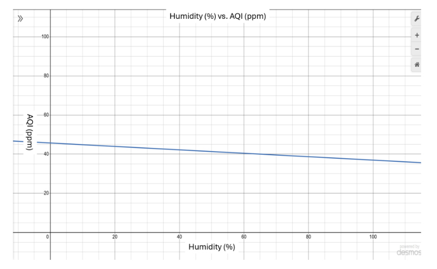
Figure 3. A graph showing the linear regression model of the calculated slope of humidity and AQI. As humidity increases, AQI decreases.

Figure 4. A graph showing the linear regression model of the calculated slope of temperature and AQI. As temperature increases, AQI decreases.

Discussion/Conclusion

These results do not support our expected hypothesis for temperature, pressure, and humidity, and our background research does not support our results. Pearson correlations indicate that temperature and pressure have significant negative correlations with AQI, while humidity does not. This could suggest problems in our study such as a non-optimal data collection period. These results do not correlate to the other studies and trends that were cited in the Introduction section of our paper. Humidity has the least effect on the state and density of air, and therefore its ability to hold pollutants. Humidity only increases the moisture in the air and does not have as significant of an effect when compared to temperature and pressure, and has less of an effect on the pollutant levels. Temperature is directly related to wildfires and other emissions from pollutant producing sites such as factories or mobile sources, like cars. As the temperature of air increases the heat and radiation, the levels of other pollutants in the atmosphere and PM2.5, can as well. The spread of a growing wildfire may not only increase the amount of PM2.5 and other sizes of PM in the air, but also the surrounding temperature in the air. This may have increased the temperature and the particulate matter readings surrounding our sensors when we collected data. Additionally, the time period of our data included a period of wildfires on the West Coast.

This could have increased the PM2.5 and temperature readings from all the surrounding sensors, while decreasing the humidity readings by an even larger margin. Whereas this may not have skewed the entire dataset to decrease the significance of humidity’s impact on AQI, some western sensors may have had lower humidity data than they would have without the wildfires. However, it is not possible to compare this data because there is no benchmark of data without wildfires present, as the weather is constantly changing and the data is being collected in real time. As for pressure, it would be understandable that higher levels may create more concentrated pollutants because there is more stagnant air. This stagnant air usually does not allow the pollutants to move or circulate to different areas, or diffuse into the rest of the atmosphere, which creates masses of air that have much higher concentrations of pollutants, as opposed to areas of lower pressure.

The linear regressions (Fig. 2,3,4) that were generated by Microsoft Excel and then by Desmos’ graphing calculator, make it seem like there is the same positive correlation between AQI and all three variables. However, this is not true, as shown in the Pearson correlations (Table 1), because while all variables may have a negative correlation in the linear regressions, they do not all have a significant enough relationship for a p<0.05. This is why the regressions look like they have the same slopes, when they really are not the same level of significance.

As for future studies, either the PurpleAir network or an alternative method of data collection could be used to establish further correlations between temperature, pressure, humidity, and air quality. Future research could either corroborate or contradict our findings and may align with current understanding of correlations from other studies. For example, a future study could be an experiment all year round, consisting of all four seasons, fall, winter, spring, and summer, rather than only collecting data for six weeks across two seasons, summer and fall. With a shorter time period of data collected, possible confounding variables could have altered our results. A year round experiment may eliminate these confounding variables and create a data collection period that could account for seasonal fluctuations in these factors. Another example of a future study could be where the cross seasonal fluctuations are further analyzed and more concrete correlations could be understood for air quality levels across seasons. This can contribute to many aspects of science and society that were not previously capitalized upon. Now, citizens of cities around the world can contribute to their atmospheric profile and environmental knowledge through PurpleAir and the correlations that we established. By identifying environmental drivers of air quality, policymakers and citizens can better anticipate and respond to pollution events, ultimately reducing health risks.

---

Written by Angelica Zinytche, Veronica Zinytche, and Jack Cohen

Acknowledgments

We thank Dr. Holler for his guidance and instruction. We also thank Fordham University for providing resources, including PurpleAir.

References

• PurpleAir, Inc. (n.d.). Real-time air quality monitoring by PurpleAir.

• https://www2.purpleair.com/

• Daouda, M., et al. (2022). Racial/ethnic disparities in nationwide PM2.5 concentrations: Perils of assuming a linear relationship. Environmental Health Perspectives, 130(7). https://doi.org/10.1289/ehp11048

• Liu, J., Clark, L. P., Bechle, M., Hajat, A., Kim, S.-Y., Robinson, A., Sheppard, L., Szpiro, A. A., & Marshall, J. D. (2021). Disparities in air pollution exposure in the United States by race-ethnicity and income, 1990–2010. https://doi.org/10.26434/chemrxiv.13814711

• Larr, A. S., & Neidell, M. (2016). Pollution and climate change. Future Child, 26(1), 93–113. http://www.jstor.org/stable/43755232

• Manisalidis, I., Stavropoulou, E., Stavropoulos, A., & Bezirtzoglou, E. (2020). Environmental and health impacts of air pollution: A review. Frontiers in Public Health, 8, 14. https://doi.org/10.3389/fpubh.2020.00014

• New York State Department of Environmental Conservation. (n.d.). Home. https://dec.ny.gov/

• Qurratulain, S. T., & Khwaja, M. A. (2019). Health effects due to poor ambient air quality (AAQ). In Assessment of Pakistan National Ambient Air Quality Standards (NAAQS’s) with Selected Asian Countries & WHO (pp. 8–11). Sustainable Development Policy Institute. http://www.jstor.org/stable/resrep24367.7

• Spickett, J. (2024). Climate change and air quality: The potential impact on health. https://www.jstor.org/stable/26723789

• Nordström, K., Andersson, L. M., Lindvall, P., & Blomquist, J. (1994). Effect of air humidification on the sick building syndrome and perceived indoor air quality in

• CORRELATIONS BETWEEN AQI LEVELS OF PM2.5 IN THE UNITED STATES AND TEMPERATURE, ATMOSPHERIC PRESSURE, AND HUMIDITY 15

• hospitals: A four-month longitudinal study. Occupational and Environmental Medicine, 51(10), 683–688. http://www.jstor.org/stable/27730196

• Education, UCAR Center for Science. (2024). How weather affects air quality. Center for Science Education. https://scied.ucar.edu/learning-zone/air-quality/how-weather-affects-air-quality

• Education, UCAR Center for Science. (2024b). Extreme events and human health. Center for Science Education.

• https://scied.ucar.edu/learning-zone/climate-change-impacts/extreme-events-and human-health